The following is some extremely simple code to show pcolor handles
matrices and matrices with latitude information.
% Read in the NCEP - NCAR Reanalysis sea-level pressure (SLP) data (mb) fn = 'slp.mon.mean.nc' xgrid = nc_varget( fn, 'lon' ); ygrid = nc_varget( fn, 'lat' ); nx = length(xgrid) ny = length(ygrid) fdat = nc_varget( fn, 'slp' ); % Calculate the grand mean SLP. gmean = squeeze(mean(fdat)); whos fdat gmean xgrid ygrid % fdat 749x73x144 62987904 double % gmean 73x144 84096 double % xgrid 144x1 576 single % ygrid 73x1 292 single clf pcolor( gmean ); set( get(gca,'Children'), 'EdgeColor', 'none' ) colorbarGridpoint gmean(1,1) is centered at 90N,0E; and "pcolor" assigns this to the lower left position on the plot. The high SLP values at the top of the plot are actually for Antarctica.
clf pcolor( xgrid(:)', ygrid, gmean ) set( get(gca,'Children'), 'EdgeColor', 'none' ) colorbarIncluding the latitude information as an input to "pcolor" gets the routine to assign Southern Hemisphere values to the bottom half of the plot, and Northern Hemisphere values to the top half of the plot. Todd Mitchell, June 2010

load worldlo  % A geography data base
worldlo  % Provides information on what is in the data base
figure
axesm( 'eqdcylin','MapLatLimit',[ -40 10 ], 'MapLonLimit', [ -85 -30 ]+360 )
h = displaym( POline );     % POlitical boundaries and coastlines as lines.
set( h(1), 'Color', ones(1,3)*0.7 );  % Make the borders and coasts gray.
set( h(2), 'Color', ones(1,3)*0.7 );
framem

% Plots some circles and Xs for station locations
h1 = plotm( raob, 'ko', 'MarkerSize', 10 );
h2 = plotm( sonet, 'kx', 'MarkerSize', 10 );
Todd Mitchell, October 2000.

I have done this without the toolbox functions.  I'm sure that it can
be done with the toolbox, but I can't easily tell you how.  If you
know, please add this information.

% Read in an elevation data set.  Several reside at
% /home/disk/tao/data/elevation/

clf
% I shade the continents with "landmask" which was written by Alexis
% Lau.  I'm sure that the MATLAB toolbox also does this, but I don't
% know how.  To use Alexis' routine, typing for following into your
% MATLAB session should work.
/home/disk/tao/bantzer-work/matlab/lau/link_alexis_scripts.m

landmask( ones(1,3)*0.9 );
hold on

% The following routines requires the field plotted (the elevations)
% to be a two-dimensional matrix, and longitude and latitude
% information ("xmat" and "ymat", respectively) to be of the
% same dimensions.  I want to contour the 200 and 1500m elevations.
[ c, h ] = contour( xmat, ymat, elevmat, [200 1500], 'k-' );
% Each line segment is described with a "handle".  Change
% the specification of each line segment so that the lines are gray
% and thick.
for ih = 1: length(h)
if get( h(ih), 'UserData' )==200
set( h(ih), 'Color', ones(1,3)*0.7 )
else
set( h(ih), 'Color', ones(1,3)*0.5, 'LineWidth', 0.4 );
end
end

% Plot station locations as circles.
plot( raob(:,2), raob(:,1), 'ko', 'MarkerSize', 5 );
Todd Mitchell, October 2000
How to write lots of text outside of the plot.
This is not a mapping toolbox issue, but it is very useful!

axes('position',[0,0,1,1]);  % Define axes for the text.
% In this case, the axes are for the entire page.
% Write some text:
htext = text(.5,0.1,'blah, blah, blah', 'FontSize', 14  );
% Specify that the coordinates provided above are for the middle
% of the text string:
set(htext,'HorizontalAlignment','center');
set(gca,'Visible','off');

axes('position',[0.25,0.3,0.5,0.5]);  % Define axes for the plot or map.
plot( randn(10,1) );  % Plot something.
Thanks to Meghan Cronin of PMEL for showing me this. Todd Mitchell,
November 2000.
Land and ocean masks using the mapping toolbox.
% Define something to plot (a matrix of the latitudes).
xgrid = [ 2.5: 5: 360 ]' ;
ygrid = [ 87.5: -5: -87.5 ]' ;
nx = length(xgrid)
ny = length(ygrid)
xval = ones(ny,1)*(xgrid');
yval = ygrid*ones(1,nx);

% Ocean mask
% Define a map projection, in this case cylindrical.  Specify domain.
axesm('eqdcylin','MapLatLimit',[ 20 80 ], 'MapLonLimit', [ -170 -50 ]+360 )
% Shade the field of interest.
contourfm( yval, xval, yval ); shading flat
% Apply the mask.
h3 = displaym(worldlo('oceanmask'));
set(h3, 'Facecolor', [ 1 1 1 ] );
set(h3, 'Edgecolor', 'none' );
caxis( [ -87.5 87.5 ] )
colorbar


% To mask out everything, but the contiguous U.S., you need to
% do a few more things.
% There are several matlab supplied data sets:
% worldlo, worldhi, oceanlo, usalo, and usahi; and each of these
% is comprised of several data structures.  To find out the
% structures, type either "help data_set_name" or just "data_set_name"
% and it will show you the structure names.  You will need the data
% structures in order to mask out states, countries, and selected
% geographical features (the Great Lakes).

% For identifying countries to mask, you need "worldlo" (or maybe
% "worldhi" would do)
load worldlo POpatch
% loads the "POpatch" structure from the "worldlo" data set.
POtags = {POpatch.tag};
canada = POpatch(find(strcmpi(POtags,'canada')));
greenland = POpatch(find(strcmpi(POtags,'greenland')));
mexico = POpatch(find(strcmpi(POtags,'mexico')));
cuba = POpatch(find(strcmpi(POtags,'cuba')));

% Similarly, to obtain the structure for Alaska
load usalo state
statetags = {state.tag};
alaska = state(find(strcmpi(statetags,'alaska')));

% Now you can, mask out states and countries:
h = displaym([canada, greenland, mexico, cuba, alaska]);
set(h, 'FaceColor', [1 1 1 ], 'EdgeColor', [1 1 1 ]);


% As a bonus, one of the data sets has a Great Lakes structure.
load usalo greatlakes
g = displaym(greatlakes); set(g,'Facecolor',[0 0 1],'EdgeColor',[0 0 1]);


% Land mask
clf
axesm('eqdcylin','MapLatLimit',[ 20 80 ], 'MapLonLimit', [ -170 -50 ]+360 )
contourfm( yval, xval, yval ); shading flat
h3 = displaym(worldlo('POpatch'));
set(h3, 'Facecolor', [193 153 103]/256 );
set(h3, 'Edgecolor', 'none' );
caxis( [ -87.5 87.5 ] )
colorbar

Todd Mitchell,
December 2000.
Controlling shading intervals and colors.
Matlab is quite happy to choose shading intervals and color scheme for you. With a little work, however, you can actually specify the colors and shading intervals yourself.
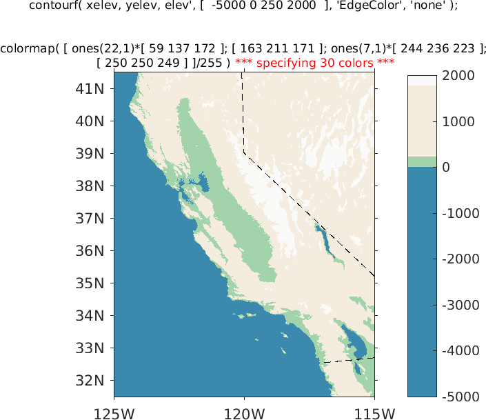
% Contourf takes the minimum and maximum contour values you
% specify, assigns the minimum value to colormap row 1 and the maximum
% value to the last row of the colormap, and linearly interpolates the
% colors for all of the other contours.  This is a problem if your shading
% intervals vary.

% In the above, the shading jumps are at  -5000 0 250 2000.
% The lowest shading level is specified to be -5000, which is *** less ***
% than the minimum value in the data to be plotted.  If the minimum
% contour specified is greater than the lowest value to be plotted,
% contourf will shade it white.

% To get the colormap to work, I chose the contours to be divisible by 250
% and the number of colors I specified is equal to ( maximum - minimum ) / 250 + 1
% This works !!!!!
Todd Mitchell, September 2018.
Making movies
"help movie" and "help getframe" will give you all of the details. The following is just the essential code.
m = moviein(last-first+1);
plot the data
for time = first: last
clf
m(time) = getframe;
To show the movie:
end
movie( m, [ #_times_to_show_movie first:last ], frames_per_second )
To save the movie outside of the Matlab session:
movie2avi( m, filename.avi );
Todd Mitchell, April 2010
Plotting an image
Sometimes you want a plot where you can pick off data values for individual cells.
"pcolor" is awful, but you can modify the plot with a lot of work to make it serviceable. In the following I had a table where values range from 0 to 5. I wanted 0 to plotted as white and 5 to be red.
pcolor( [ yr1:yr2 ], [ 1: 62 ], temp' );
h2 = colorbar( 'vert' )
set( h2, 'YTickLabel', '' );
colormap( [ ones(1,3); flipud( prism(5) ) ] );
set( gca, 'TickDir', 'out' )
set( get(gca,'Children'), 'EdgeColor', 'none' );  % turns off the grid
set( gca, 'YLim', [ 0 63 ] );
set( gca, 'YTick', [ 0:5:60 ] );
set( gca, 'XLim', [ 1848 2012 ] );
set( gca, 'XTick', [ 1850:10:2010 ] );
set( gca, 'XTickLabel', [ '1850'; '    '; '1870'; ...
  '    '; '1890'; '    '; '1910'; '    '; '1930'; ...
  '    '; '1950'; '    '; '1970'; '    '; '1990'; ...
  '    '; '2010'; '    ' ] );
hold on
for xval = 1850:10:2010
h = plot( [ xval xval ], [ 1 62 ], 'k-' );
set( h, 'Color', ones(1,3)*0.8 );
end
for yval = 5:5:60
h = plot( [ 1850 2010 ], [ yval yval ], 'k-' );
set( h, 'Color', ones(1,3)*0.8 );
end
ylabel( 'station index', 'FontName', 'Times', 'FontSize', 14 );
title( '# of June through October months contributing (0-5)', ...
  'FontName', 'Times', 'FontSize', 18 );
Todd Mitchell,
January 2008
Controlling contour label fonts and sizes.
The Matlab routines "contour" and "contourm" draw contours, the latter on maps. One of the outputs of these scripts is the "contour matrix" and this can be used with clabel and clabelm, respectively, to plot contour labels. An example would be "h = clabel( c )," where "c" is the contour matrix output of "contourm." I plot contours on top of shaded land forms (see below) and the matlab default is for negative contour values to be plotted with a negative "ZData" value. This can cause parts of the label to be under the land mass and not visible. To fix this and, to controll the font name and size, do the following:
[ c, h ] = contour( ... );
h2 = clabel( c );
for icnt = 1: length(h2)
if strcmp( get( h2(icnt), 'Type' ), 'text' )
set( h2(icnt), 'FontName', 'Times' )
set( h2(icnt), 'FontSize', 14 )
Position = get( h2(icnt), 'Position' );
set( h2(icnt), 'Position', Position(1:2) );
end
end

Full size PNG
Todd Mitchell, July 2011.
Interpolating data with missing values (NaNs) to a new grid.
Sometimes one needs to interpolate data to a new grid. An example of this is the AVISO sea level height anomaly data, whose resolution varies with latitude. My netCDF writing routine only handles data with constant latitudinal and longitudal resolutions so I needed to interpolate the data onto a new grid. The AVISO sea level height anomaly data is only for the ocean so there are a lot of missing values to deal with.
% In "meshgrid" I input vectors of the longitude and latitude
% gridpoints for the dataset I want to create.  The outputs, xgrid2 and
% ygrid2 are longitude and latitude gridpoint arrays, respectively.
[ xgrid2, ygrid2 ] = meshgrid( [ vector of longitude points ], [ vector of latitude points ] );

fdat2 = griddata( xgrid, ygrid, fdat, xgrid2, ygrid2 );
where
  xgrid, ygrid   are arrays of the input longitude and latitude gridpoints
  fdat           is the input data array
  xgrid2, ygrid2 are the longitude and lattitude arrays, respectively,
                 for the output field.
  fdat2          is the output data array, with values interpolated at
                 the xgrid2, ygrid2 coordinates.
An easy mistake to make is to inconsistently specify the western or
eastern hemisphere in the longitude inputs to griddata. If you are specifying western longitudes as negative in xgrid, you
have to do the same in xgrid2. Messing this up can yield an
interpolated field of zeros, and several hours of frustration.
Using color in a figure title
It is sometimes elegant to use color in figure titles:

PNG | PS
title( '{\color{blue}low}, mean, and {\color{red}high}'
  );
enables you to do this. A clever user named "Phonon" at
stackoverflow.com posted how to do this. Gracias.
You can also specify the rgb values of the colors, as in:title( [ '500mb \omega (Pa/s, RAP)' char(10) ... '# lightning strikes in 256 km^2:' ... '{\color{red}1-2 }{\color[rgb]{0 .4 .0}5+ }' ... '{\color[rgb]{0.8 0.4 0}10+ } (WWLLN)' ] );
Plotting contours on top of shading
clf
[ c, h ] = contourf( xgrid, ygrid, temp, [  1: 7  ], 'EdgeColor', 'none' );
colorbar( 'southoutside' );
cLim = get( gca, 'CLim' );
hold on
contour( xgrid, ygrid, temp2, [ -1.5: 0.25: -0.25 ], 'k-' );
contour( xgrid, ygrid, temp2, [ -0.25/2 -0.25/2 ], 'r-' );
set( gca, 'CLim', cLim );
will produceWithout the "set( gca, 'CLim', cLim )" call, colorbar will use the contour information from the contour plots.
Contolling labels on shading
Matlab has an awful shading labeling convention of marking the jump in shading with a + mark, and writing the data value of the jump off to the side. To get rid of the + marks, and to put the labels on the jumps in shading:

[ c, h ] = contourf( ... );
ti = clabel( c,  'FontSize', 14 );
% "ti" has an even number of rows, and each label is associated with a
% two rows of information.  I turn off the + mark by setting the
% "Marker" attribute to "none"; extract the + mark position from the
% first row; and modify the label, including its position, in the second row.
for icnt = 1: length(ti)/2
    set( ti((icnt-1)*2+1), 'Marker', 'none' )
    XData = get( ti((icnt-1)*2+1), 'XData' );
    YData = get( ti((icnt-1)*2+1), 'YData' );
    set( ti((icnt-1)*2+2), 'Position', [ XData YData 0 ] );
    set( ti((icnt-1)*2+2), 'HorizontalAlignment', 'center' );
    set( ti((icnt-1)*2+2), 'VerticalAlignment', 'middle' );
end
The above as a matlab function, "fixcontourlabels.m".
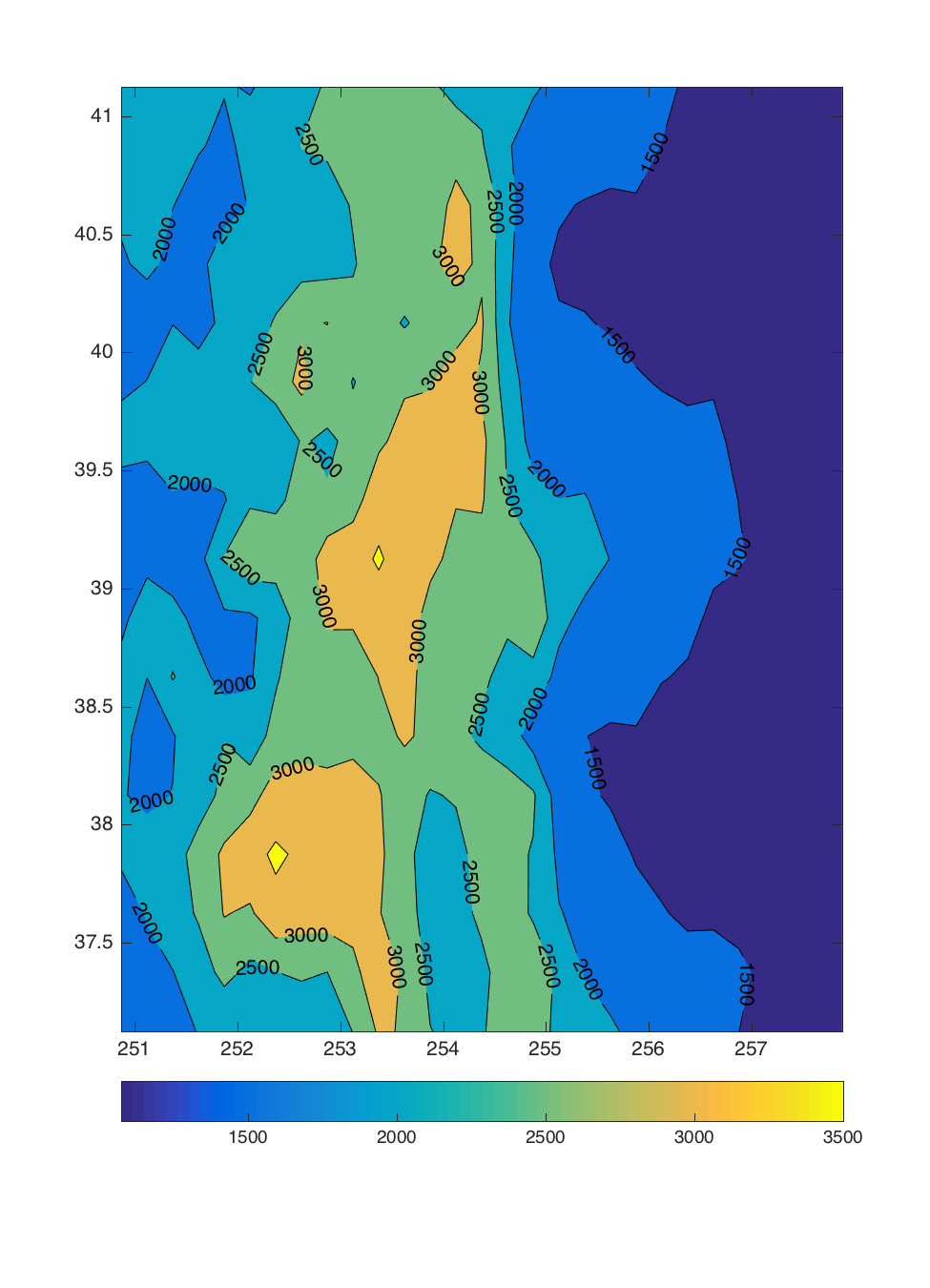
Choosing the contourf minimum contour and making the colorbar consistent with the plot
Consider the following simple plot produced by contourf.
load contourfdata.mat % You can read in the data: lon, lat, and elev % "elev" is an elevation dataset for Colorado, and its values range % between 1074 and 3569 meters. colormap( 'default' ) clf [ c, h ] = contourf( lon, lat, elev, [ 1000: 500: 3500 ] ); clabel( c, h ) ch = colorbar( 'location', 'SouthOutside' ); % A key ingredient in the procedure is that a contour must be % specified that is smaller than the lowest value in % "elev". In this case, a contour of 1000 is specified.There are useful MATLAB documentation pages on colorbars and graphics object properties
The above code produces the plot on the left. The plot has jumps in color and the colorbar is a continuum range of colors. If the plot contours weren't labeled, you would have to guess the values plotted. % The following code will modify the colorbar to produce one that is % consistent with the plot. contours = get( h, 'LevelList' ) nshade = length(contours); colorint = floor( 64 / nshade ) % The default colormap has 64 colors. cmap = colormap; colormap( cmap(1:colorint:end,:) ) % Use a smaller number of colors in the colorbar % Modify the minimum and maximum values used in the colorbar. caxis( [ contours(1)-(contours(2)-contours(1)) ... contours(end)+(contours(end)-contours(end-1)) ] ); set( ch, 'Ticks', contours(2:end) ); % Get rid of the leading color in the colorbar (which isn't used) Limits = get( ch, 'Limits' ); set( ch, 'Limits', [ Limits(1)*2 Limits(2) ] ); font( 'Times', 12 )

Use "convert" to crop an image

"Convert" is a command line utilty maintained by ImageMagick.org.

1) convert -trmm fnin fnout

will pretty severely trim the white space from around the plot.

You can use "eval" to perform this operation from within MATLAB:

eval( [ '!convert -trim ' fnin ' ' fnout ';' ] )
you need the spaces in this command for it to work.

2) convert -crop WxH+X+Y fnin fnout

where W and H: the desired width and height of the cropped image
        in mystery unts, respectively
      X and Y: retain the cropped image beginning this many mystery units
        from the left and top borders, respectively
      fnin and fnout are the input and output image filenames,
        respectively, and may be the same.
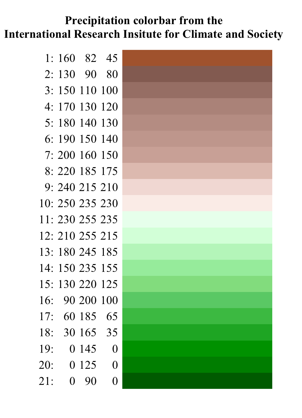
An ascii file of the RGB values courtesy of Michael Bell of the IRI.
Multiple plots on the same page
axes( 'Position', ... ) is used to accomplish this. The results of get( gcf, 'Position' ) are [ 0.1300 0.1100 0.7750 0.8150 ] which are the shift from the left (l), shift from the bottom (b), width (w) , and height (h) of the plot. For each new plot, call axes( 'Position', [ l b w h ] ) at the beginning of the specification of the plot. It worked better if the height is much less than 0.8150. This method was also used to put text outside of the plot (above).
How contourf picks colors
I plot latitudes to see how contourf picks colors.
contourf( x, y, y, [ 45: 49 ] )

contourf( x, y, y, [ 45 46 47:0.5:48 49 ] )

Gridding irregularly spaced data
I have tried to use interp2( lon, lat, data, xq2, yq2 ),
without success. One gets the following error message:
Error using griddedInterpolant
The grid vectors are not strictly monotonic increasing.

Error in interp2>makegriddedinterp (line 228)
    F = griddedInterpolant(varargin{:});

Error in interp2 (line 128)
        F = makegriddedinterp({X, Y}, V, method,extrap);

The solution is to use
interpolant = scatteredInterpolant(lon, lat, data);
where lon, lat, and data are vectors

dataq = interpolant(xq2, yq2);
where xq2 and yq2 are matrices that define the gridpoints you want interpolated values at.