by J. M. Wallace
Notes by: Eric DeWeaver and Michael Palmer
Both the Northern and Southern Hemispheres have leading modes of
circulation variability with deep, barotropic, zonally symmetric
structures. We refer to these modes as the Arctic and Antarctic
Oscillations (AO/AAO), or more generically as annular modes. This
talk gives a historical perspective on the modes, and documents their
spatial patterns in temperature, sea level pressure (SLP), and
zonal-mean zonal wind ([u]). While the AO is defined as a monthly-mean,
extratropical, tropospheric pattern of variability, its influence
extends well beyond these categories. As will be shown below, it has
connections to extreme weather events and long-term climate trends, a
distinctive signature in the tropics, and important connections to the
stratosphere.
Dave Thompson, who has been the driving force behind much of the
recent activity related to the AO and AAO, has put together an
informative webpage on annular modes, which can be found at
http://tao.atmos.washington.edu/data/annularmodes .
Anyone wishing further information on annular modes or more detail
on the material presented here should consult this webpage.
Why do we like ring-like modes? There are several reasons that we
might expect annular modes to figure prominently in the low-frequency
behavior of the atmosphere. First, it is well known (e.g. Pedlosky
1987) that vorticity conservation leads to an upscale energy cascade
in barotropic fluids, so that large-scale patterns evolve from
small-scale isotropic turbulence. In the case of rotating fluids,
Rhines (1975; see also Pedlosky 1987) showed that the upscale cascade
leads to the development of strong zonally elongated zonal jets.
Also, zonally oriented eddies propagate more slowly than meridionally
oriented eddies of the same size, so zonal structures -- and
particularly zonally symmetric patterns, which do not disperse as
Rossby waves at all -- should be more prominent in the time mean.
Second, the studies by Lorenz (2000) and DeWeaver and Nigam (2000)
show that [u] anomalies can generate anomalous eddies which provide
further momentum to sustain the original [u] anomalies. This positive
feedback means that annular anomalies are likely to persist longer
than regional anomalies.
Third, numerical models provide evidence that annular modes are easily
excited by external forcing. Byron Boville found that the circulation
in the winter stratosphere in CCM0 was extremely sensitive to changes
in the radiation code. He found that a zonal-eddy feedback was
important in establishing the circulation changes, which had an
annular structure extending from the stratosphere to the ground.
Shindell et al. (1999) found similar circulation changes in the
response of their model to anthropogenic greenhouse gas forcing. They
characterized the response as an excitation of the positive phase of
the AO.
The beast that we refer to as the AO or the Northern Hemisphere
annular mode (NAM) has been characterized in different ways by
different researchers. The principal schools of thought are
summarized in figure 1. One group of researchers, starting with
Walker and Bliss (WB, 1932) and including van Loon and Rogers (1978) and
Hurrell (1995), regarded the phenomenon as a regional climate
variation and referred to it as the North Atlantic Oscillation (NAO).
A parallel effort, including work by Rossby, Willett, and Namias,
studied esssentially the same variability by looking at fluctuations
of the zonal-mean circulation. They defined various zonal indices to
identify this variability, which they regarded as fundamentally
zonally symmetric or annular. Finally, a third group, including
Kutzbach (1971), Trenberth (1981), and Wallace and Gutzler (1981),
characterized the dominant mode of Northern Hemisphere variability
using the leading EOF of SLP. Like these authors, we use the leading
SLP EOF to define the AO (Thompson and Wallace 1998, 2000; Thompson et
al. 2000).
The regional perspective of WB may be less a deliberate decision
than a consequence of the limited data available at the time. The top
panel in figure 2 shows the spatial pattern of the NAO from WB, while
the bottom panel shows the spatial pattern that results when their NAO
index is reconstructed using a modern data set (see Wallace 2000 for
details). As you can see, the pattern takes on a much stronger
circumpolar aspect when a more comprehensive data set is used. Given
more complete data, Walker and Bliss might have called their pattern
the AO rather than the NAO.
Rossby (1939) introduced the zonal index as a measure of the change
in strength of the midlatitude westerlies. However, this idea was
revised by Namias (1950), who proposed that index fluctuations were
really changes in the meridional position of the zonal jet rather than
its strength. In the high phase of the index, the jet is shifted
towards higher latitude, the polar vortex is intensified, and cold air
is walled off in the polar vortex. In the low phase, the vortex is
weaker, the jet is shifted southward, and cold air outbreaks are more
common. Lorenz (1951) considered the variability of Northern
Hemisphere SLP, and showed that pressure tends to be out of phase
between high and low latitudes. He suggested that an index made by
averaging [u] at 55N (U55) would serve as a good measure of this
pressure variability. A similar index, called the ``polar pressure
deficit'', was constructed by Gates (1950), who took the average SLP
from 45N to the north pole and subtracted it from the zonal-mean SLP
at 45N.
Despite their differing regional and circumpolar perspectives, the
patterns produced by NAO and zonal indices are quite similar. Figure
3 shows the correlation between SLP at each gridpoint and the
two-point Portugal - Iceland NAO index (i.e., SLP in Iceland minus SLP
in Portugal), Lorenz's U55 index, and the leading EOF of SLP. All
three are highly correlated, and all show opposition between pressure
over the polar cap and the subpolar belt.
It follows that the NAO and AO are synonyms: they are different names
for the same variability, not different patterns of variability. The
difference between the terms is in whether that variability is
interpreted as a regional pattern controlled by Atlantic sector
processes or as an annular mode whose strongest teleconnections lie in
the Atlantic sector. The AO is also the embodiment of what earlier
researchers have called the Northern Hemisphere ``index cycle''.
To examine the signature of the AO in SLP, [u], and surface and
midtropospheric temperature, we regress these fields against the
standardized time series for the AO, formed by calculating the leading
EOF of SLP from 20N to 90N. The regression of [u] and SLP against the
AO time series is shown in figure 4. For this figure the AO time
series is generated using all months of the year, but January,
February, and March make the largest contributions to the patterns.
Note that the Pacific SLP center is much more prominent here than in
the correlation map in figure 3. The correlation is weak, but the
North Pacific is a region of high variance, so the center shows up
with greater amplitude in the regression map.
The [u] regression shows that when pressure is low over the pole and
high in the subpolar belt, abnormally strong westerlies show up north
of 45N. The westerly anomalies are accompanied by easterly anomalies
which are centered on 35N but extend into the tropics at low levels,
where they can be viewed as a strengthening of the trades. The trade
strengthening occurs mostly in the Atlantic sector, but there is a
small Pacific contribution as well. The tropical easterlies extend
from the surface to the jet stream level, and westerly anomalies
overly the easterlies at high levels in the deep tropics.
The Antarctic Oscillation is the dynamical twin of the AO, and it
can be calculated as the leading EOF of SLP or 850mb height from 20S
to the south pole. The patterns of [u] and SLP regressed against the
AAO time series, shown in figure 5, have much in common with the AO
patterns. Again we see a polar low surrounded by a high pressure
belt, and a deep dipole pattern in [u]. By superimposing the AO and
AAO plots, you can see the high level of agreement in the [u] patterns
for the two hemispheres. The level of agreement is even higher if the
AAO regression is done just for November and December, because in that
season the AAO [u] anomalies extend strongly into the stratosphere.
An important aspect of AO variability is its connection to surface air
temperature (SAT). Figure 6a shows the SAT pattern for the AO from
the Comprehensive Ocean-Atmosphere Data Set (COADS), and figure 6b
shows the corresponding land SAT from the Global Historical
Climatology Network (GHCN). By superimposing the two you can see that
the high phase of the AO (low pressure over the pole) is accompanied
by cold temperatures over eastern Canada and Greenland, while warm
conditions prevail over Siberia and the United States in the subpolar
belt.
The tropospheric temperature anomalies of the AO and AAO extend well
into the tropics, and even across the equator. Figure 7a shows the
tropospheric temperatures from John Christy's MSU 2LT data set. As in
the surface temperatures, cold temperatures over Greenland are
surrounded by a warm ring. But the figure also shows that the cold
pole is accompanied by a slight cooling of the global tropics (in 7a
and 7b the colors saturate so that the weak tropical temperature
anomalies are visible). The same banded structure is evident for the
AAO: the tropics are cold when the pole is cold. Figure 7b shows the
Pacific half of the temperature patterns.
Figure 8 summarizes the features of the AO in its high index phase,
defined as the polarity in which the subpolar westerlies are
anomalously strong. In this phase, a cold low sits over the pole,
surrounded by a belt of enhanced westerlies at 55N, which is
accompanied by a slackening of the westerlies around 35N. Warm high
pressure conditions prevail between 35N and 55N, and cold anomalies
occur in the tropics, accompanied by a strengthening of the trades.
In addition, high level westerlies appear over the equator. The [u]
dipole in the extratropics is accompanied by a mean meridional
circulation which acts to decelerate the upper-level [u] anomalies
through Coriolis torque. The anomalies are maintained against the
torque by convergence of eddy momentum fluxes, represented by the thick
arrows. At the surface, the mean meridional circulation acts in the
opposite sense, maintaining the [u] anomalies against friction and
enhancing the surface trades.
In addition to these features, low ozone values occur in the high
latitude stratosphere during the high index phase. The low values can
be understood as a consequence of a reduction in the strength of the
stratospheric Lagrangian mean circulation. The Lagrangian mean
circulation transports ozone from the tropical stratosphere to the
pole, so any reduction of the circulation serves to deplete ozone at
high latitudes.
The key features in figure 8 can be explained in terms of wave
refraction. In midlatitudes, upward propagating Rossby waves are
refracted more or less strongly towards the tropics, depending on the
strength of the lower stratospheric polar vortex. In the low AO
phase, the polar vortex is weak, so more waves are refracted into it.
When these waves break they decelerate the vortex even more. In the
high phase the strong vortex refracts more wave activity into the
tropics, and the breaking of these waves transports momentum into the
vortex, making it stronger. This feedback is illustrated
schematically in figure 9, in which the thin arrows represent the
Eliassen-Palm flux of planetary waves and the contours show the
strength of the westerlies.
The thick arrows show the Lagrangian mean circulation in the
stratosphere, also known as the Brewer-Dobson circulation. This
circulation is always poleward in the Northern Hemisphere, driven by
wave breaking and diabatic cooling in the polar vortex. In the high
index phase of the AO, there is less wave breaking in the polar vortex
and the Lagrangian mean circulation is weaker, while the opposite
holds in the low index phase. Since the Brewer-Dobson circulation is
responsible for bringing ozone into the polar stratosphere, the amount
of ozone in the polar stratosphere depends on the strength of the
circulation.
The schematic in figure 8 suggests that there will be coupling
between the tropospheric AO and conditions in the lower stratosphere,
and evidence for this coupling is presented by Baldwin and Dunkerton
(1999). They form a multi-level AO pattern by taking the leading EOF
of 90-day low-pass geopotential height north of 20N at five levels
(1000, 300, 100, 30, and 10 hPa), and using regression against the EOF
time series to obtain the AO pattern at all available levels from 1000
to 10hPa. The AO pattern at each level is then projected onto the
filtered data for the level, and the projection coefficients are
plotted in figure 10 as a function of time and height. In the figure,
red (blue) represents above (below) average geopotential height in the
polar cap. The figure shows a significant correlation between the
troposphere and the stratosphere, with a tendency for signals to
propagate downward. Thus the troposphere feels the influence of the
stratosphere, although it's not clear whether this relationship is
strong enough to be a useful forecasting tool.
Figure 11 documents the AO's effect on the motion of Arctic sea
ice. The figure, adapted from Rigor et al. (2000), shows the movement
of Arctic sea ice during low (top) and high (bottom) AO phases. The
vectors come from an objective analysis of buoy data for the period
1979-98. In the low phase, there is a great deal of recirculation in
the clockwise ``Beaufort gyre'', which enhances sea ice thickness by
allowing the ice to remain in the cold central Arctic, growing thicker
from year to year. Also, the clockwise circulation causes more
rafting and piling up of the ice due to Ekman convergence, again
making thicker ice floes. On the other hand, the high AO phase leads
to a reduction in the recirculation and shorter ice residence times.
Meanwhile, reduced advection from the Canadian side promotes opening
of the ice on the Russian side, and there is an increase in the
passage of ice through Fram Strait and out into the North Atlantic.
Thus the AO can have a strong effect on Arctic sea ice thickness.
The GHCN precipitation anomalies associated with the AO are shown
in figure 12. Wetter conditions prevail throughout most of the
Arctic, while drier conditions occur in southern Europe. Of
particular interest to those of us at the University of Washington are
the wetter conditions along the Pacific coast from Oregon to Alaska.
Blocking has a lot to do with the severity of winter weather in the
Northern Hemisphere, and the AO has a strong ability to control
blocking. To quantify this control, we define a blocking event as a
week or more of excess pressure in the midtroposphere together with an
anticyclone at the surface. By this definition, figure 13 shows that
blocking occurs preferentially during the low AO phase in Alaska, the
North Atlantic, and Russia. In the North Atlantic, there is no
blocking at all in the high AO phase. A strong control in the North
Atlantic is to be expected, given the strength of the AO signal there,
but even in Alaska there is a two to one preference for blocking in
the low AO phase.
In fact, the AO influences all indicators of severe weather to some
extent, as can be seen from the statistics compiled in the next two
figures. Figure 14 gives a sample of regions which have a much higher
incidence of cold days during the low index. For instance, minimum
temperatures less than -15C in Yakima, Washington are much more likely
on low index days than on high index days, a fact which may be of some
interest to the fruit growers there. Figure 15 shows a preference for
the low AO phase in blocking days, cold surges, cold temperatures,
frozen precipitation, and strong winds and waves in a variety of
locales throughout the northern extratropics.
In addition to its importance for monthly-mean variability, blocking,
and severe weather events, the AO has played a substantial role in the
climate trends of recent decades. To show this we first plot the AO
time series from the 1860s to the present in figure 16. The top curve
shows a time series for the AO based on its signature in the SAT,
while the bottom curve is the AO based on SLP data. In the top curve
the SAT comes from the Jones et al. (1999) data set, and the backward
reconstruction is largely determined by the Siberian SAT data. In the
bottom curve, the blue color shows a reconstruction from the 1870s to
1932 using WB's NAO index (a combination of SLP and SAT at several
stations). In both panels it is clear that AO has been on the rise
since the 1960s, although there appears to be a decadal signal
superimposed on the upward trend (the decadal signal is not correlated
with the sunspot cycle). Since the AO is the leading mode of climate
variability in the Northern Hemisphere, the climatic consequences of
this trend are clearly of interest. The suite of figures that follows
documents these consequences in a variety of important indicators of
climate and atmospheric circulation.
The 30-year JFM trend in SLP is shown in the top panel of figure 17,
while the bottom panel shows the AO's contribution to that trend. In
the 30 years from 1968 to 1997, SLP over the Arctic has dropped 6 to
10 mb, while SLP over the North Atlantic and western European sectors
has risen. Comparison of the top and bottom panels reveals that the
AO makes an impressive contribution to these changes. The only place
where the total trend differs from the AO pattern substantially is in
the North Pacific, where ENSO-like decadal variability is the dominant
player (e.g. Trenberth and Hurrell 1994, Zhang et al. 1997).
Likewise, the 30-year wintertime trend in zonal-mean circulation is
strongly influenced by the AO. Figure 18 shows that the JFM [u]
trend, with changes of up to 9m/s in stratospheric wind speed, is
virtually identical to the AO [u] pattern. A similar result holds for
the AAO in the Southern Hemisphere. The 30-year [u] trend in the
Southern Hemisphere is plotted in figure 19 for the months of November
and December, the months when the AAO [u] anomalies extend into the
stratosphere. The [u] trend strongly resembles the AAO anomalies,
although there are some uncertainties regarding the quality of the
Southern Hemisphere data for the earlier years of the record.
The AO also makes a substantial contribution to [T], as shown in
figure 20. However, the polar stratospheric temperature has decreased
dramatically, and the AO contribution to the trend does not account
for all of this decrease. The radiative effect of ozone depletion
must also be involved.
Figures 21 and 22 display the SAT trend and SAT regressed against the
AO index, respectively. The AO contributes to the warming of Siberia
and the cooling of Greenland and the Middle East. Overall, the AO
accounts for over 30% of the JFM warming of the Northern Hemisphere
continents (more details can be found in Thompson et al. 2000).
Precipitation trends and AO-related precipitation anomalies are shown
in figures 23 and 24. In both figures there is drying in southern
Europe and the Sahel. A tendency for wetter conditions is also found
in both plots extending inland from the Pacific coast of Alaska and
throughout much of central Asia. The disagreement over China is
partly due to the influence of decadal ENSO-like variability.
A table of the AO contribution to various climate indicators is
presented in figure 25, listing contributions to SAT, SLP, rainfall in
Norway and Spain, column ozone, and MSU4 lower-stratospheric
temperature. In all cases, the AO contribution is substantial.
As discussed above (figures 8 and 9), the AO influences wintertime
stratospheric ozone concentrations by modulating the Lagrangian mean
stratospheric circulation. Thus one would expect the upward trend in
the AO to lead to some ozone depletion, and this expectation is
confirmed in figure 26. The top panel gives the column ozone trend in
Dobson units for March 1979-1993, and the bottom panel gives the AO
contribution to the trend. March is the relevant month because the
sun rises over the Arctic in March. Arctic Ozone observations are not
available during the polar night, and photochemical ozone depletion
occurs primarily in March. The AO contribution bears a strong spatial
resemblance to the total trend, and accounts for about half of its
amplitude and much of its spatial structure.
Changes in Arctic sea ice movement also have a strong component
congruent with the AO, as can be seen from figures 27 and 28. Figure
27 shows ice movement regressed on the AO, while figure 28 shows the
difference in ice movement between the periods 1989-1998 and
1979-1988, taken from Rigor et al. (2000). The figures show that the
AO is linked to a reduction in the strength of the Beaufort gyre
recirculation (see figure 11). Also, the difference vectors have an
component outward through Fram Strait, and this component increases
with the AO. The AO is thus implicated in the thinning of the Arctic
sea ice reported by Rothrock et al. (1999).
Since the high frequency variability of the AO is much greater than
its decadal variability, it is appropriate to think of the change in
the AO as a preference for the positive phase rather than a steady
increase over time. A measure of this preference is given in figure
29, which shows the number of days with positive or negative AO
anomalies exceeding one standard deviation for the decades 1958-67 and
1988-97. In the earlier period, low index AO days exceeded high index
AO days by a factor of two in JFM, while in the more recent period
high index days exceeded low index days by a factor of six.
Surprisingly, the change in preference is also evident in summer
(JJA), with low days exceeding high days by a factor of two for the
earlier period, and the opposite ratio in the later period.
Finally, we consider the influence of the AO on the breakdown of
the Northern Hemisphere polar vortex at the end of the winter season.
In the positive AO phase the vortex tends to be stronger, so a
positive AO trend in late winter implies an extension of the
stratospheric winter season. The delay of the spring breakdown was
demonstrated by Zhou et al. (2000), who have kindly contributed figure
30. In this figure, the fraction of the world covered by the polar
vortex is plotted for the 650K, 550K, 450K, and 400K (approximately
20, 40, 80, and 120mb) isentropes over the course of the seasonal
cycle. At all four levels, it can be seen that the breakup of the
polar vortex happened later in 1992-98 (red curve) than in 1980-85
(black curve) or 1986-91 (blue curve). According to these curves, the
winter season in the stratosphere has been extended by about two
weeks.
The figures presented here highlight the differences between the AO
and NAO nomenclature. To be sure, most of the statistical
relationships are strongest in the North Atlantic sector. But it may
be more useful to think of the dynamics in terms of zonal-mean cross
sections, such as in figure 9, which depicts the interplay of the
zonal-mean flow and the planetary wave fluxes. Also, the AO has a
dynamical twin in the Southern Hemisphere, the AAO. The AO
terminology highlights the analogous nature of the two structures,
while the NAO terminology would suggest that we look for a South
Atlantic Oscillation, or perhaps a North Pacific Oscillation. It must
also be emphasized that although the AO has its strongest centers in
the North Atlantic, its influence is at least hemispheric in scope, as
can be seen from the broad tropical cooling in the MSU 2LT regressions
and the enhancement of the trade winds. Furthermore, the AO's effect
on blocking is felt throughout the hemisphere. Finally, the
zonal-mean perspective is helpful for thinking about interactions
between the stratosphere and the troposphere.
1. Introduction
2. Motivation
3. Perspectives on the Northern Hemisphere annular mode
4. AO and AAO signatures in atmospheric and surface variables
5. The AO's effect on blocking and extreme weather events
6. The AO and climate change
7. Concluding remarks
References
Note: All figures shown here can be downloaded as postscript files.
To access a postscript file, click on the corresponding image.
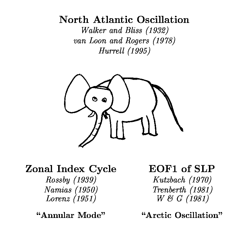
Figure 1
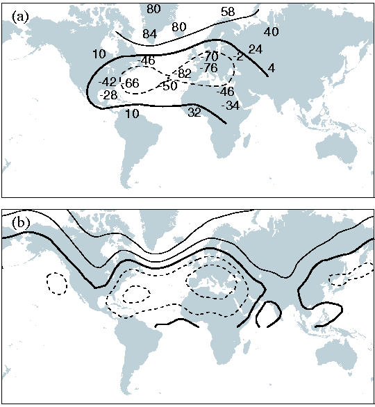
Figure 2
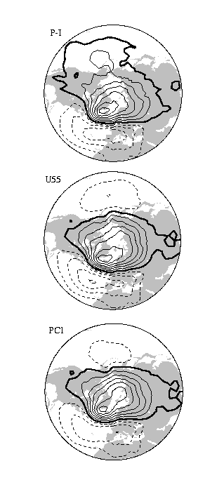
Figure 3
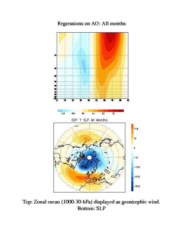
Figure 4
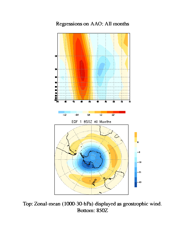
Figure 5
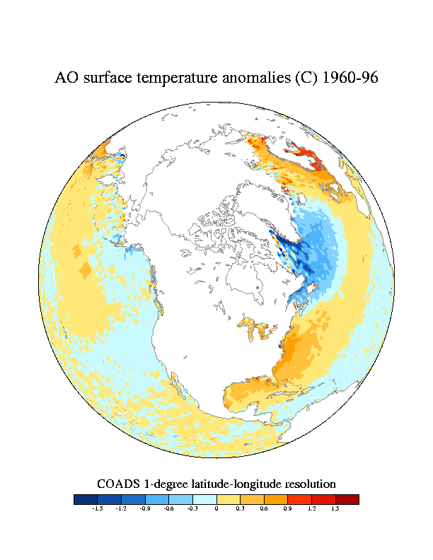
Figure 6a
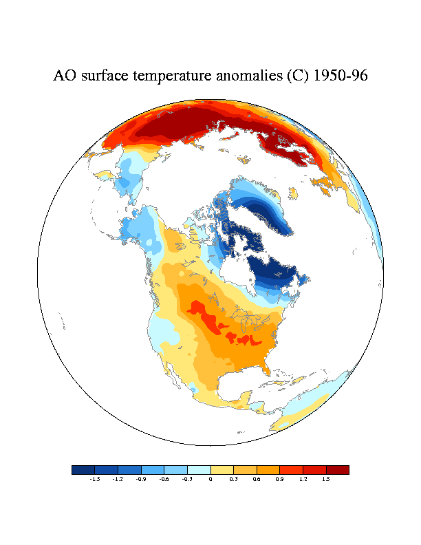
Figure 6b
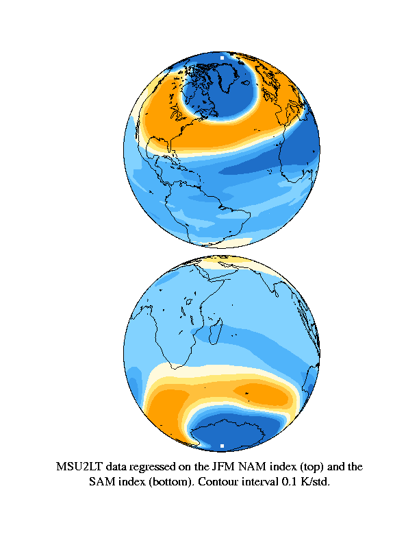
Figure 7a
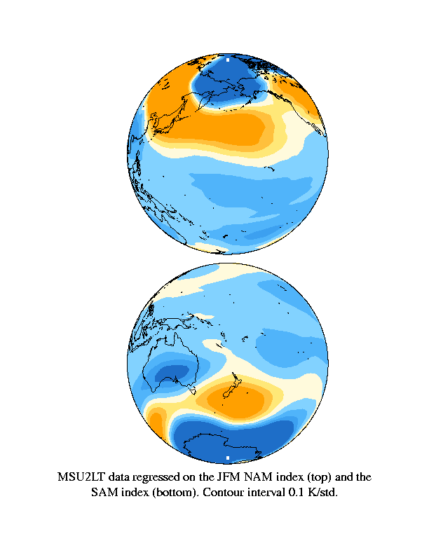
Figure 7b
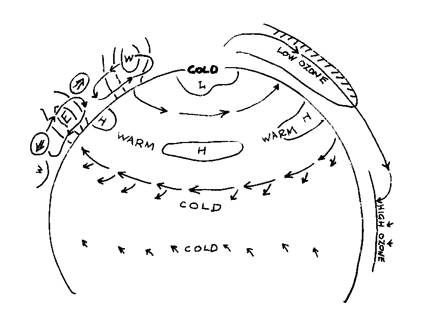
Figure 8
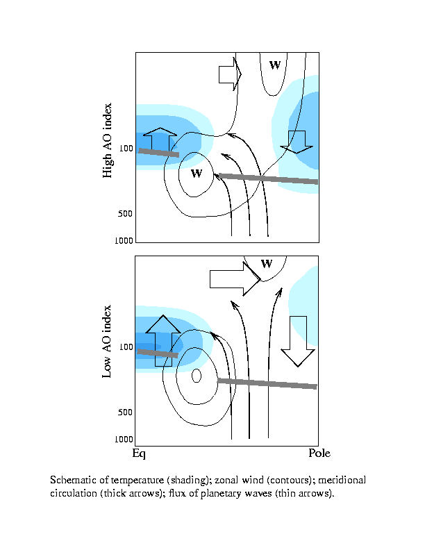
Figure 9
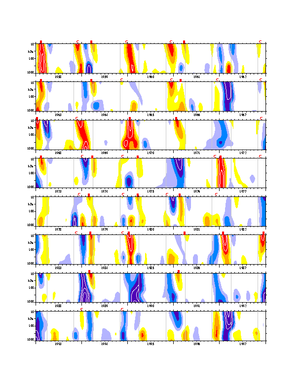
Figure 10
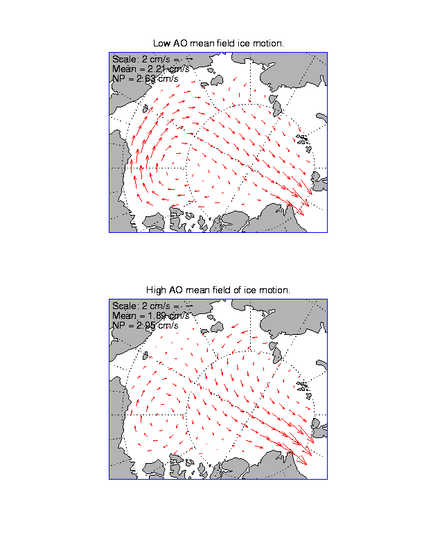
Figure 11
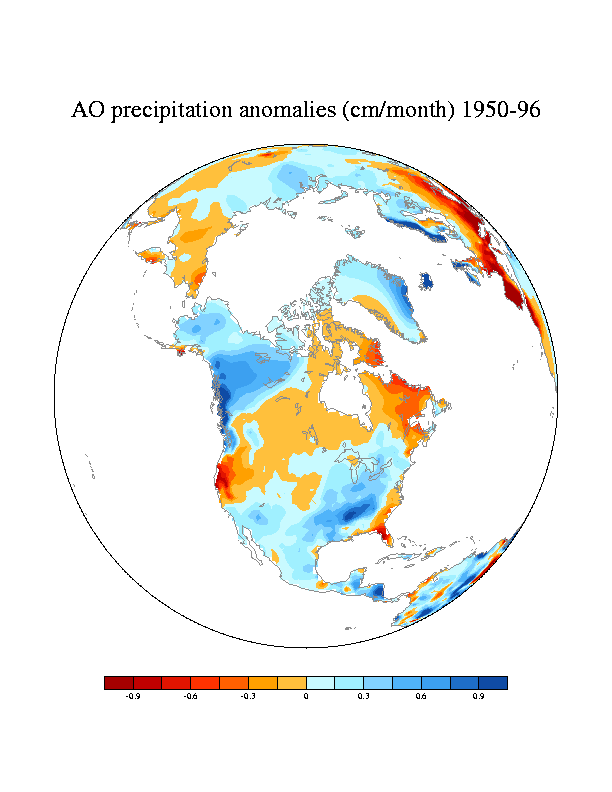
Figure 12
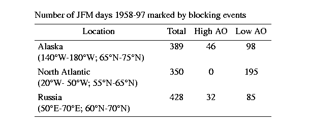
Figure 13
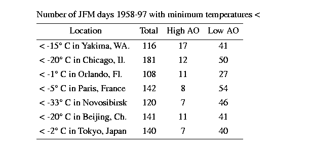
Figure 14
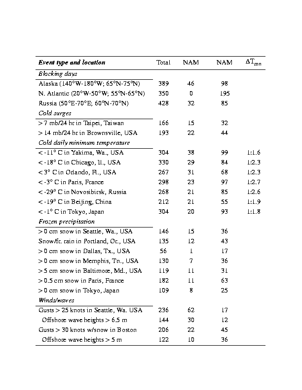
Figure 15
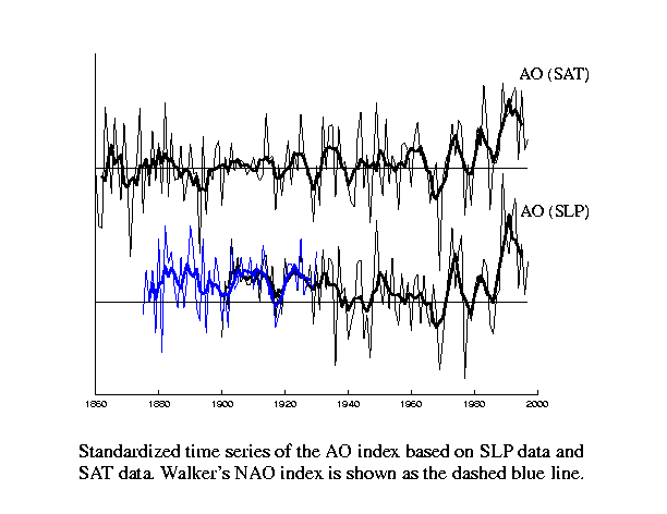
Figure 16
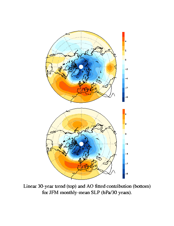
Figure 17
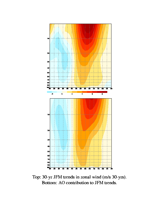
Figure 18
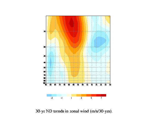
Figure 19
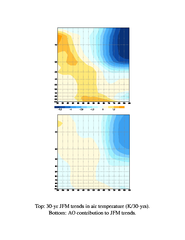
Figure 20
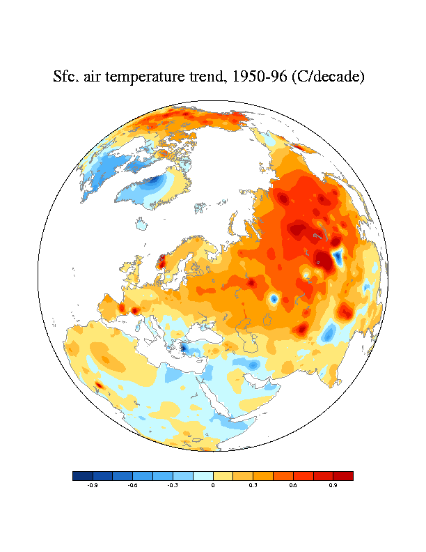
Figure 21
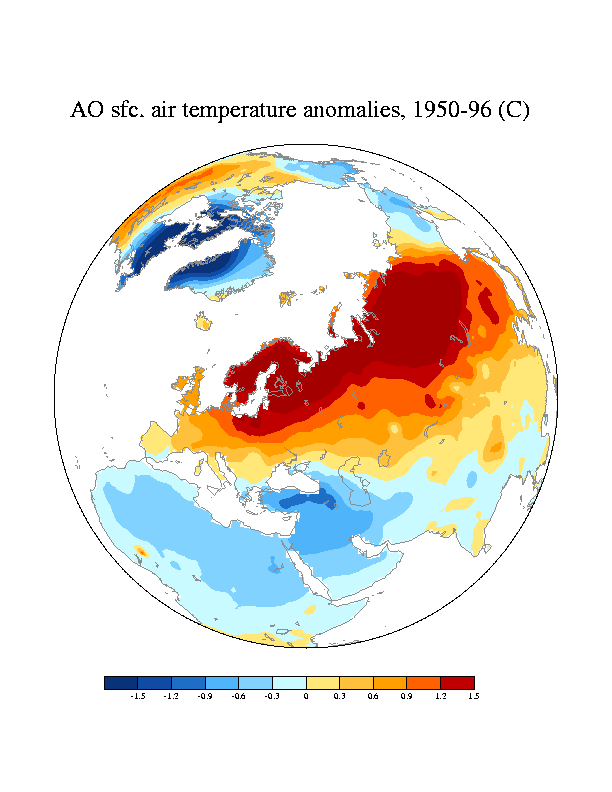
Figure 22
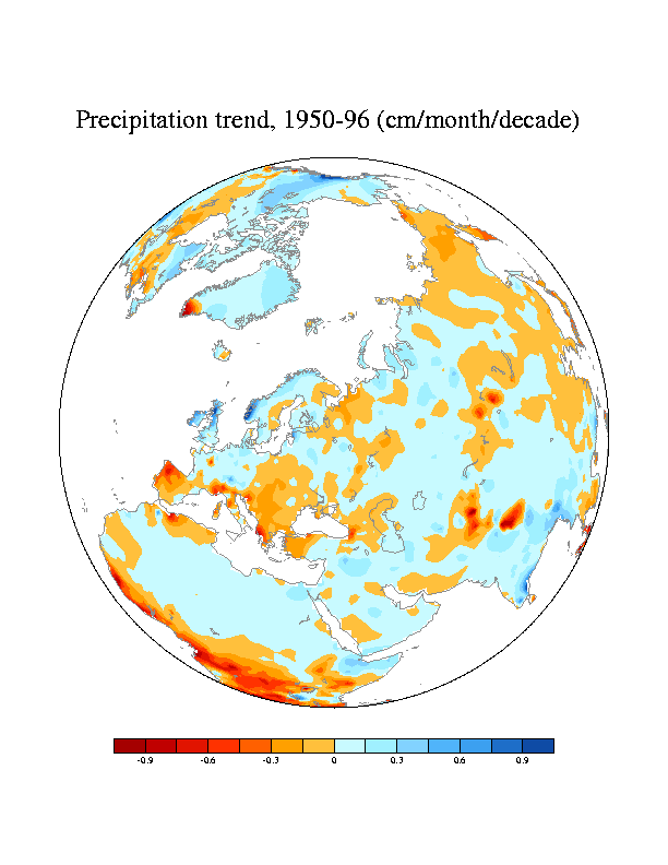
Figure 23
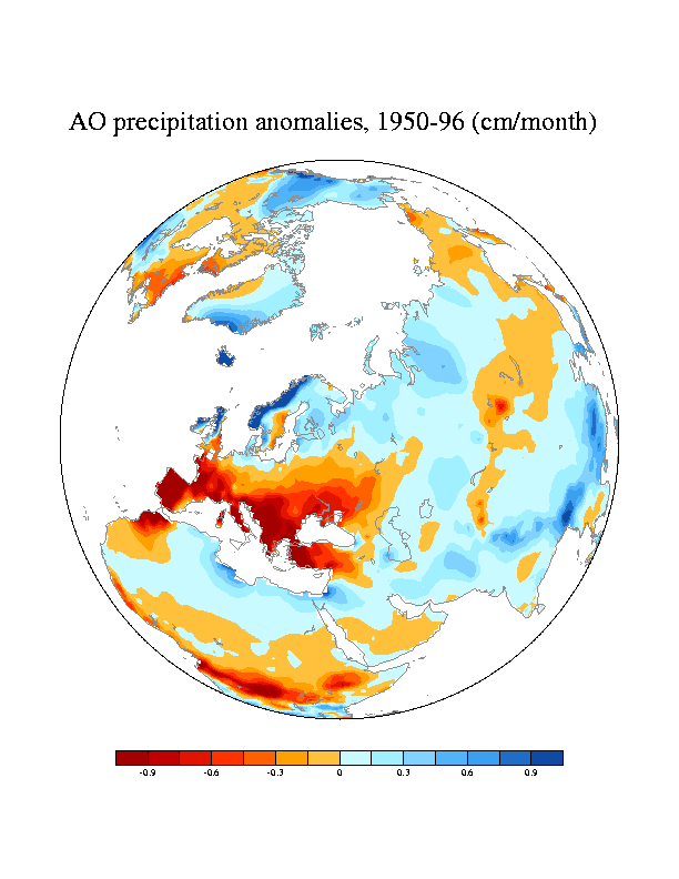
Figure 24
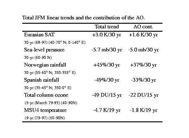
Figure 25
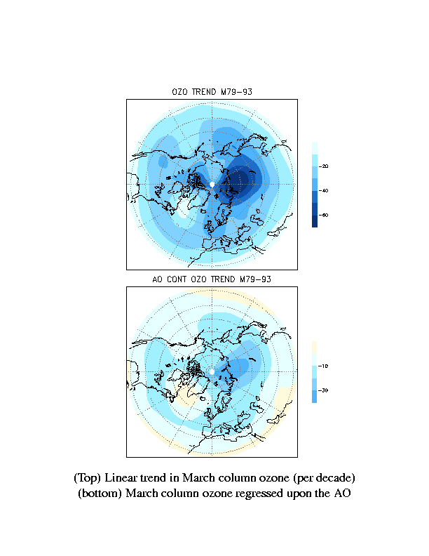
Figure 26
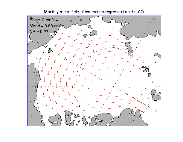
Figure 27
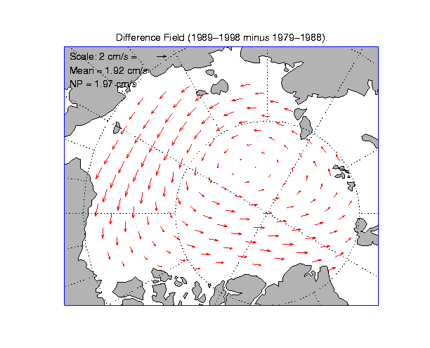
Figure 28
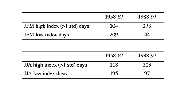
Figure 29
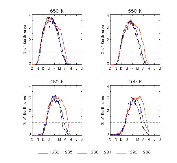
Figure 30